Part 3: Adaptive Rounding: GPTQ

In my last post, I covered Optimal Brain Quantizer (OBQ). OBQ breaks quantization into per-layer, row-wise subproblems: at each step it quantizes the weight that adds the least error, then compensates the remaining unquantized weights using a proxy Hessian. The catch is scalibility - the greedy search runs in $O(d^2)$ per row (at each step you evaluate all remaining weights), and since different rows quantize in different column orders, they require separate Hessian copies to parallelize, making the algorithm memory-bound at scale.

In this post, we look at GPTQ, one of the most widely used methods for weight only quantization of LLMs, and the first to demonstrate 3-bit quantization of LLMs is also viable. GPTQ came from the same lab as OBQ and is built directly on it. The authors did a deep dive analysis of the bottlenecks in OBQ and introduced a set of algorithmic optimizations that made it significantly faster. Together, these optimizations reduced the computational overhead of OBQ substantially, allowing GPTQ to scale to models as large as 175B parameters, which the authors report quantizing in approximately 4 hours.

Generative PreTrained Transformer Quantization (GPTQ):¶

Let’s discuss the main insights of GPTQ that made OBQ practical at scale:

Observation 1: Aribtrary Order Insight¶

The first observation made by GPTQ was that the gap between greedy order and an arbitrary fixed order is negligible, especially at large model scales. The intuition: in greedy order, easy weights get quantized first, leaving the hard weights (those in sharp regions of the loss landscape) for last, when the few remaining weights are available to absorb the compensation error. This observation justifies quantizing weights in a simple left-to-right column order. This means we can eliminate the greedy $O(d^2)$ search step for every row & more importantly, it allows us to parallelize the process across rows without needing copies of the Hessian.

Observation 2: Lazy Batch Updates¶

Consider a naive implementation of OBQ for a 4906 x 4096 matrix, using the arbitrary order insight from GPTQ:

Arbitrary Order Insight GPTQ

Round column 1. Calculate the rounding error $\Delta w_1$.
Apply the compensate to columns 2 through 4096.
Update the inverse Hessian
Round column 2. Calculate $\Delta w_2$.
Apply the compensation to columns 3 through 4096.
Update the inverse Hessian
Repeat for all remaining columns.

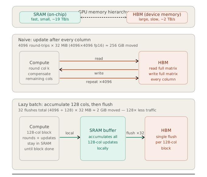
This implementation is extremely in-efficient on the GPU. At steps 2, 5, 8 . . . you load the entire weight matrix from HBM(device memory), apply a small correction, and write it back - 4096 times in total. The compute per trip is tiny, and almost all the time is spent on memory traffic. In other words, the process is memory-bound.

The key thing to realize is that we don’t need to immediately flush each correction to the full matrix. A column that won’t be quantized for another 100 steps doesn’t need its update yet. So, we can be lazy and defer these global updates. GPTQ processes a block of 128 columns entirely within SRAM, accumulating all corrections locally, and only then flushes the result to HBM in a single write. This reduces the memory traffic by 128x.

Lazy Batch Update

Observation 3: The Cholesky Reformulation¶

Next, the authors found repeatedly updating the inverse Hessian, especially for large models containing large number of columns, leads to catatrophic numerical inaccuracies, i.e the floating point arthimatic errors accumulate & degrade the Hessian leading to garbage update of weights.

The key thing to realize here is that the weight update only ever reads from one row of $\mathbf{H}^{-1}$ at a time. Specifically, row $p$ after weight $p$ has been quantized:. Recall,

$$ \Delta w_{\text{remaining}} = \Delta w_p \frac{ \left(\mathbf{H}^{-1}\right)_{p,\ \text{remaining}} }{ \left(\mathbf{H}^{-1}\right)_{pp} }. $$

What if we had a matrix that already contained these rows in a numerically stable form, so we could read them off sequentially and skip the rank-one update entirely?

It turns out that the rank-one update:

$$ H^{-1}_{-p} = H^{-1} - \frac{1} {\left(H^{-1}\right)_{pp}} H^{-1}_{:,p} H^{-1}_{p,:}, $$

is how fast linear algebra libraries calculate the Cholesky Decomposition with a minor change. So instead of updating $\mathbf{H}^{-1}$ repeatedly, we can compute the Cholesky factorization of $\mathbf{H}^{-1}$ once upfront:

$$ \mathbf{H}^{-1} = \mathbf{L}\mathbf{L}^\top $$

and read off row $p$ of $\mathbf{L}$ at each quantization step.

With all the three observations in place, the full GPTQ algorithm is:

Algorithm GPTQ

Iterate through the network one layer at a time.
Run the calibration dataset through the network and collect input activations $\mathbf{X}$ for the current layer.
Compute the proxy Hessian with a dampening factor $\lambda$ for numerical stability:
$$ \mathbf{H} = \mathbf{X}\mathbf{X}^{\top} + \lambda\mathbf{I}. $$
Compute the Cholesky factorization of $\mathbf{H}^{-1}$:
$$ \mathbf{H}^{-1} = \mathbf{L}\mathbf{L}^{\top}. $$
Initialize an error buffer $\mathbf{E} \in \mathbb{R}^{d_{\mathrm{row}} \times B}$ with zeros. This buffer accumulates the rounding errors within each block.
For each block of $B$ columns of the weight matrix:
1. For each column $p$ in the block:
  1. Quantize the weight vector $\mathbf{w}_p$ and compute its rounding error:
    $$ \Delta\mathbf{w}_p = \hat{\mathbf{w}}_p - \mathbf{w}_p. $$
  2. Store $\Delta\mathbf{w}_p$ in the corresponding column of $\mathbf{E}$.
  3. Update the remaining FP16 weight vectors inside the block using $\Delta\mathbf{w}_p$ and the corresponding row of $\mathbf{L}$. These updates remain in SRAM.
Flush the accumulated updates to the remaining columns outside the block using a single matrix multiplication:
$$ \mathbf{W}_{:,\mathrm{remaining}} \leftarrow \mathbf{W}_{:,\mathrm{remaining}} - \mathbf{E}\mathbf{Q}, $$
where $\mathbf{Q}$ is the corresponding $B \times d_{\mathrm{remaining}}$ submatrix of $\mathbf{L}$.
Move to the next layer and repeat.

Conclusion¶

Thank you for reading! I hope the post helped demystify GPTQ — one of the most widely adopted weight-only quantization methods, and the one that first demonstrated viable 3–4 bit quantization of large language models at scale. In the next post, we’ll look at LDLQ from QuIP. See you there!

Here’s a quick summary of GPTQ’s design choices:

Bit-width	Granularity	What’s quantized	What’s not quantized	Compute precision	Scheme
3–4 bit (typical)	Per-row; per-group (groupsize=128 common)	Weights only	Activations, KV-cache	FP16	Asymmetric uniform (default)