Part 1: Adaptive Rounding: Adaround

Adaptive rounding techniques are one of the best ways to get more accuracy from quantization with the same bitwidth. In this series we’ll cover the evolution of adaptive rounding techniques starting from Adaround which delivers excellent quality with small models to more recent ones like GPTQ, OmniQuant, FlexRound which extend the idea to models with billions of parameters. First, let’s start with building some intuition about what adaptive rounding is and why rounding direction matters at all.

Motivation¶

Recall how quantization is performed. Starting from a real-valued tensor \(x\), we map it onto an integer grid \(\{x_{\text{int}}^{\min}, \ldots, x_{\text{int}}^{\max}\}\):

where

• \(s\) is the scale
• \(z\) is the zero-point (offset)
• \(\lfloor \cdot \rceil\) denotes rounding to the nearest integer

Finally, the quantized value is reconstructed as

This procedure simply rounds every floating-point value to its nearest point on the quantization grid.

However, as it turns out, rounding to the nearest integer is not necessarily the optimal choice. To demonstrate this, the authors of AdaRound performed an interesting experiment. They quantized only the first layer of a ResNet-18 model and, instead of always rounding to the nearest integer, they generated 100 different stochastic rounding assignments, evaluated each one, and compared them against conventional round-to-nearest quantization.

Surprisingly, they found that:

• 48 out of the 100 stochastic rounding choices outperformed round-to-nearest.
• The best rounding assignment improved accuracy by more than 10 percentage points over round-to-nearest!

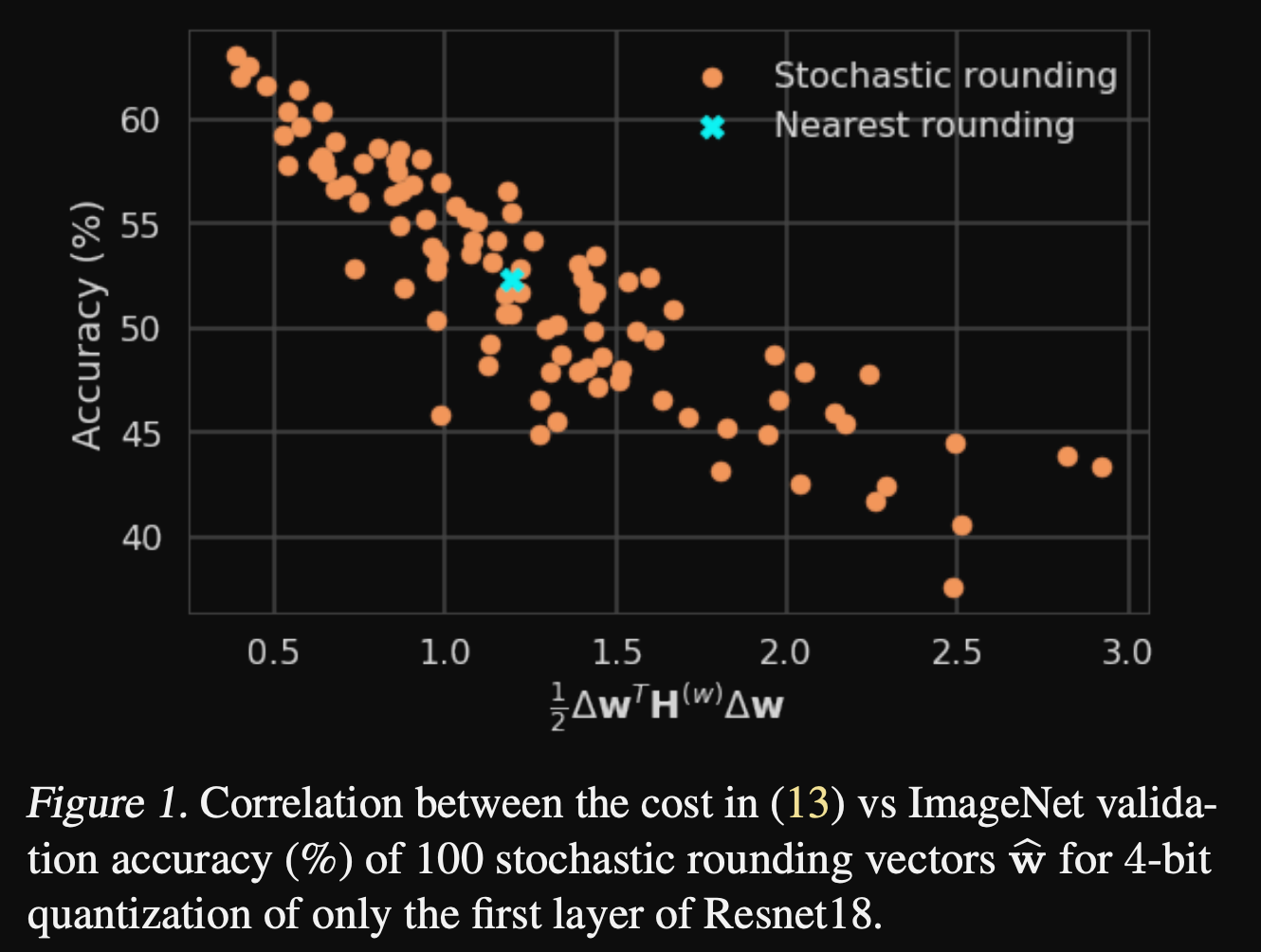
Source: Up or Down? Adaptive Rounding for Post-Training Quantization

Therefore the motivation is clear: if we can intelligently choose the rounding direction for each weight, we can often obtain substantially better quantized models without changing the bit-width.

Problem Formulation¶

The stochastic rounding experiment tells us something valuable is being left on the table by round-to-nearest, but it doesn’t tell us how to find a better rounding. Testing rounding choices by brute force is hopeless, since a single layer already has thousands of weights, each with 2 choices (round up or down).

What we need instead is a cheap, analytical way to estimate how much any given rounding choice will hurt the model’s accuracy. Before diving into the problem formulation, let’s first understand some cool math concepts which we will need for the later sections.

Prerequisites¶

1. Taylor Series Expansion¶

Taylor Series Expansion allows you to approximate any smooth function near some point \(x_0\) using only its derivatives at that point:

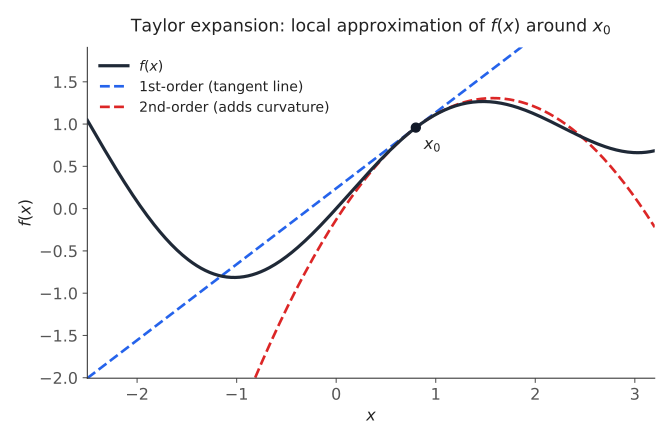
3Blue1Brown has an amazing video on Taylor Series, I would highly recommed checking it out if you want more intuition about this.

2. Hessian¶

The Hessian is just the second-order term written above. In 1D, curvature is one number, if \(f''(x)\) is positive, you’re in a bowl; if negative, a hill. In many dimensions, curvature isn’t one number anymore, because the function can curve differently depending on which direction you move. The Hessian is the matrix that holds all of these directional curvatures at once:

Diagonal entries tell you how sharply the loss curves along one weight’s own axis; off-diagonal entries tell you how curvature in one weight’s direction changes as you move along another. A 2D picture of the contour makes this easier to visualize: Notice that the two axes here curve very differently:

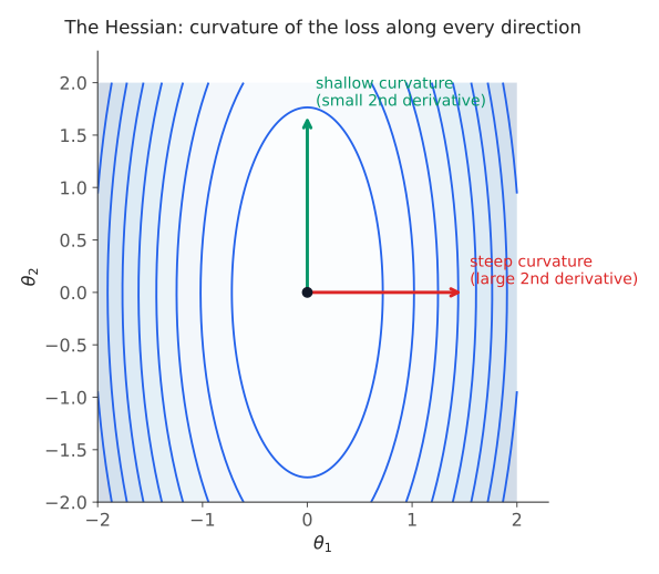
Now, let’s see how we can apply these ideas to our adaptive rounding problem.

Second-Order Analysis and Optimization¶

Quantization can be viewed as a special case of weight perturbation. Concretely, consider a neural network parameterized by the (flattened) weight vector \(\mathbf{w}\). Let \(\Delta\mathbf{w}\) denote a small perturbation to the weights (in our case, the rounding error introduced by quantization) and let \(\mathrm{L}(\mathbf{x}, \mathbf{y}, \mathbf{w})\) denote the task loss we’re trying not to disturb. What we actually care about is how much the loss changes once the weights are perturbed:

This is exactly the setting the Taylor expansion motivation from before was built for, i.e:

Since, \(\mathbf{w}\) has already converged via training, \(\mathbf{g}^{(\mathbf{w})} \approx \mathbf{0}\). So the linear term drops out, and the loss degradation from quantization is governed almost entirely by the second, Hessian-dependent term:

Layerwise Approximation¶

The Hessian-based formulation above is the starting point for many quantization and pruning algorithms, each of which has to solve the same problem: the full Hessian is infeasible to compute or store. For a network with just a million parameters, the full Hessian would have \(10^{12}\) entries and therefore computing or holding that in memory is completely infeasible.

AdaRound sidesteps this by reducing the problem to a layer-wise optimization. The underlying assumption is that minimizing the damage introduced within each individual layer is a good enough proxy for minimizing the damage to the network as a whole. Each layer’s rounding can then be optimized independently:

From Taylor Series to Local Loss¶

Even \(\mathbf{H}(\mathbf{w}^{(\ell)})\) is actually expensive to compute. Think about a single entry, the curvature between two weights \(W^{(\ell)}_{i,j}\) and \(W^{(\ell)}_{m,o}\) in the same layer. Let’s say the pre-activations are \(z^{(\ell)} = W^{(\ell)}x^{(\ell-1)}\), applying the chain rule twice gives:

Notice the structure: the result factors into a piece that only depends on which output neurons (\(i, m\)) you’re differentiating with respect to, times a piece that only depends on which input neurons (\(j, o\)) fed into them. Written for the whole layer at once, that clean factorization is exactly what a Kronecker product (\(\otimes\)) captures:

The first factor, \(x^{(\ell-1)}x^{(\ell-1)T}\), is cheap - just an outer product of the layer’s own input. The second, \(\nabla^2_{z^{(\ell)}}\mathrm{L}\), is the expensive part: it’s the curvature of the true task loss with respect to this layer’s outputs, which means backpropagating second derivatives through every layer downstream.

Adaround assumes 2 simplifications to get rid of it.

First, assume \(\nabla^2_{z^{(\ell)}}\mathrm{L}\) is diagonal, no cross-terms between different output neurons. Plugging this in, the optimization splits into one independent sub-problem per output row \(k\):

Second, assume that remaining per-row weight, \(\nabla^2_{z^{(\ell)}}\mathrm{L}_{k,k}\), is just some constant \(c_k\). A positive constant scaling one row’s objective can’t change which rounding minimizes it, so it drops out entirely, leaving:

Both simplifications together strip away every trace of the task loss and every downstream layer. What’s left is just the Mean Squared Error between the full-precision and quantized pre-activations, something you can compute from this one layer’s own inputs and outputs, with no knowledge of anything else in the network.

With that background, let’s start diving into the details of AdaRound.

AdaRound¶

AdaRound is a weight-only post-training quantization (PTQ) algorithm that learns whether each individual weight should be rounded up or rounded down.

Instead of using the standard quantization rule

AdaRound always begins by rounding every weight down using the floor operation, and then learns whether a correction of one integer step should be added.

The quantization function becomes

where

• \(V\) is a learnable parameter associated with each weight.
• \(h(V)\) is a differentiable function whose output lies in \([0,1]\).

The interpretation is straightforward:

• If \(h(V)=0\), the weight is rounded down.
• If \(h(V)=1\), the weight is rounded up.
• During optimization, \(h(V)\) can take continuous values between 0 and 1, allowing gradients to flow.

Optimization Objective¶

The authors of Adaround realized that simply minimizing the error between the original and quantized weights of an isolated layer is insufficient because the inputs to deeper layers are themselves affected by quantization errors introduced by preceding layers.

To account for this accumulated error, AdaRound uses the following asymmetric reconstruction loss:

where:

• \(W\) denotes the original weight matrix.
• \(\hat{W}\) is the quantized weight matrix parameterized by the rounding variables \(V\).
• \(x\) is the original floating-point input to the layer.
• \(\hat{x}\) is the input obtained after all preceding layers have already been quantized.
• \(f_a(\cdot)\) denotes the layer’s activation function.
• \(\lambda\) controls the trade-off between reconstruction accuracy and making hard rounding decisions.

The first term is called the asymmetric reconstruction loss. Instead of comparing the quantized layer against the original layer using identical inputs, it compares the original floating-point output \(f_a(Wx)\) against the output produced by the quantized layer operating on the actual quantized activations \(f_a(\hat{W}\hat{x})\). This more closely matches inference-time behavior and significantly reduces the accumulation of quantization errors in deeper networks.

The second term, \(f_{\mathrm{reg}}(V)\), gradually encourages every learnable rounding variable to converge toward a binary decision (round down or round up).

Let’s look at how both \(f_{\mathrm{reg}}(V)\) and \(h(V)\) are formulated.

\(f_{\mathrm{reg}}(V)\) & \(h(V)\)¶

AdaRound introduces a latent variable \(V\) for every weight, which is mapped to a soft rounding variable \(h(V)\) in [0,1] using a rectified sigmoid:

where

• \(\sigma(\cdot)\) is the sigmoid function,
• \(\gamma=-0.1\),
• \(\zeta=1.1\).

The stretched sigmoid provides a region where the gradients remain non-zero while ensuring the output is ultimately clipped to the valid range \([0,1]\).

To encourage each soft rounding decision to eventually become binary, AdaRound introduces the following regularization term:

where \(\beta\) controls the strength of the regularization.

Notice that:

• When \(h(V_i)=0\) or \(h(V_i)=1\), the regularization is zero.
• When \(h(V_i)=0.5\), the regularization is maximized.

Thus, \(f_{\mathrm{reg}}(V)\) penalizes uncertain rounding decisions while rewarding confident binary ones.

During optimization, \(\beta\) is gradually annealed from a large value (e.g., \(20\)) to a small value (e.g., \(2\)). Early on, the regularization is relatively flat, allowing the optimizer to freely explore different rounding configurations. As \(\beta\) decreases, the penalty around \(h(V)=0.5\) becomes increasingly sharp, forcing each soft decision to commit to either rounding up or rounding down.

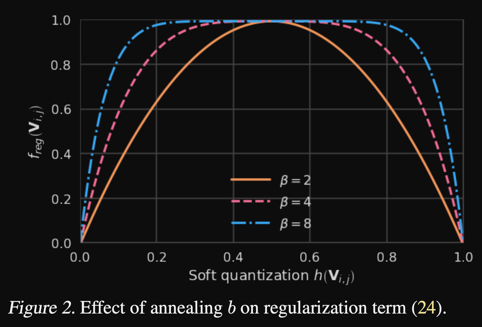Source: Up or Down? Adaptive Rounding for Post-Training Quantization

Let’s now look at the pseudo-code for Adaround:

Setup¶

1. Collect calibration data. Sample a small set of representative calibration inputs (typically a few hundred to a few thousand samples).

2. Compute layer inputs. For the current layer \(i\), compute the original floating-point input \(x\) and the quantized input \(\hat{x}\):

   • \(x\) is obtained by forwarding the calibration data through the original network;
   • \(\hat{x}\) is obtained by forwarding the same calibration data through the network where all preceding layers have already been quantized.

3. Initialize the rounding variables. Initialize the learnable rounding parameters \(V\) such that the initial soft rounding values reproduce standard nearest-neighbor rounding.

4. Initialize the regularization schedule. The regularization parameter \(\beta\) is annealed linearly throughout optimization:

   $$ \beta_t = \beta_{\text{start}} + \frac{t}{T} \left( \beta_{\text{end}} - \beta_{\text{start}} \right), $$

I’ve put together a Colab notebook implementing AdaRound from scratch and applying it to a simple MLP. I’d highly recommend working through it, as it covers the core components of a quantization framework (Observers, Quantizers, and Quantization Wrapper layers) and shows how they come together on a real network.

Limitations of AdaRound¶

AdaRound delivers excellent results across a wide range of models, from CNNs to Transformers. Its main drawback is convergence speed: AIMET’s default configuration runs 10K optimization iterations per layer for 8-bit weight quantization, and 15K iterations per layer for anything below 8-bit [1]. This makes AdaRound completely impractical for large models and where modern adaptive rounding techniques such as GPTQ step in. I’ll cover these modern techniques in future posts.

Conclusion¶

This post traced why rounding direction matters: a stochastic rounding experiment on a single ResNet-18 layer found assignments that beat round-to-nearest by over 10 points, just by choosing up vs. down more carefully. The second-order Taylor expansion showed that, for a converged network, quantization damage is governed almost entirely by the Hessian, and AdaRound makes that tractable with two simplifications (layer-wise, diagonal, constant-curvature) that collapse the objective to a simple asymmetric MSE between full-precision and quantized layer outputs. Each weight gets a learnable rounding variable, optimized layer by layer and pushed toward a hard decision by an annealed regularizer.

The cost is 10K–15K gradient steps per layer which is fine for CNNs, but completely impractical for LLMs. In the next one, we’ll look at BRECQ (Block Recontstruction Quantization) which extends AdaRound’s layer-wise reconstruction to the level of a whole block (e.g. a residual block), and argues this granularity and not layerwise or full network reconstruction gives the best trade-off between capturing cross-layer dependencies and avoiding generalization error. See you there! 👋

References¶

1. Up or Down? Adaptive Rounding for Post-Training Quantization
2. AIMET AdaRound Documentation