Why do transformers have outliers?

Modern Machine Learning models are trained with a large number of parameters, often too large, and this overparameterization is very useful during training as it creates a vast search space for the model to encode rich representations from data into its parameters. However, as it turns out, models do not use all these parameters efficiently, creating a lot of redundancy.

Training is only a short stage in a model’s life cycle and the model spends majority of its time inferencing, where this overparameterization leads to excessive memory usage, slower response times, and increased power utilization. This redundancy is precisely why model compression techniques like pruning, quantization, or low-rank decomposition can often be applied with little loss in accuracy.

Transformer models, however, contain unusually large values concentrated in certain feature dimensions of both weights and activations. These dimensions, known as outlier channels, are highly sensitive to model-compression. In this blog post, we will build intuition for why outlier channels emerge in transformer models and what drives their formation.

How Transformer Models Work¶

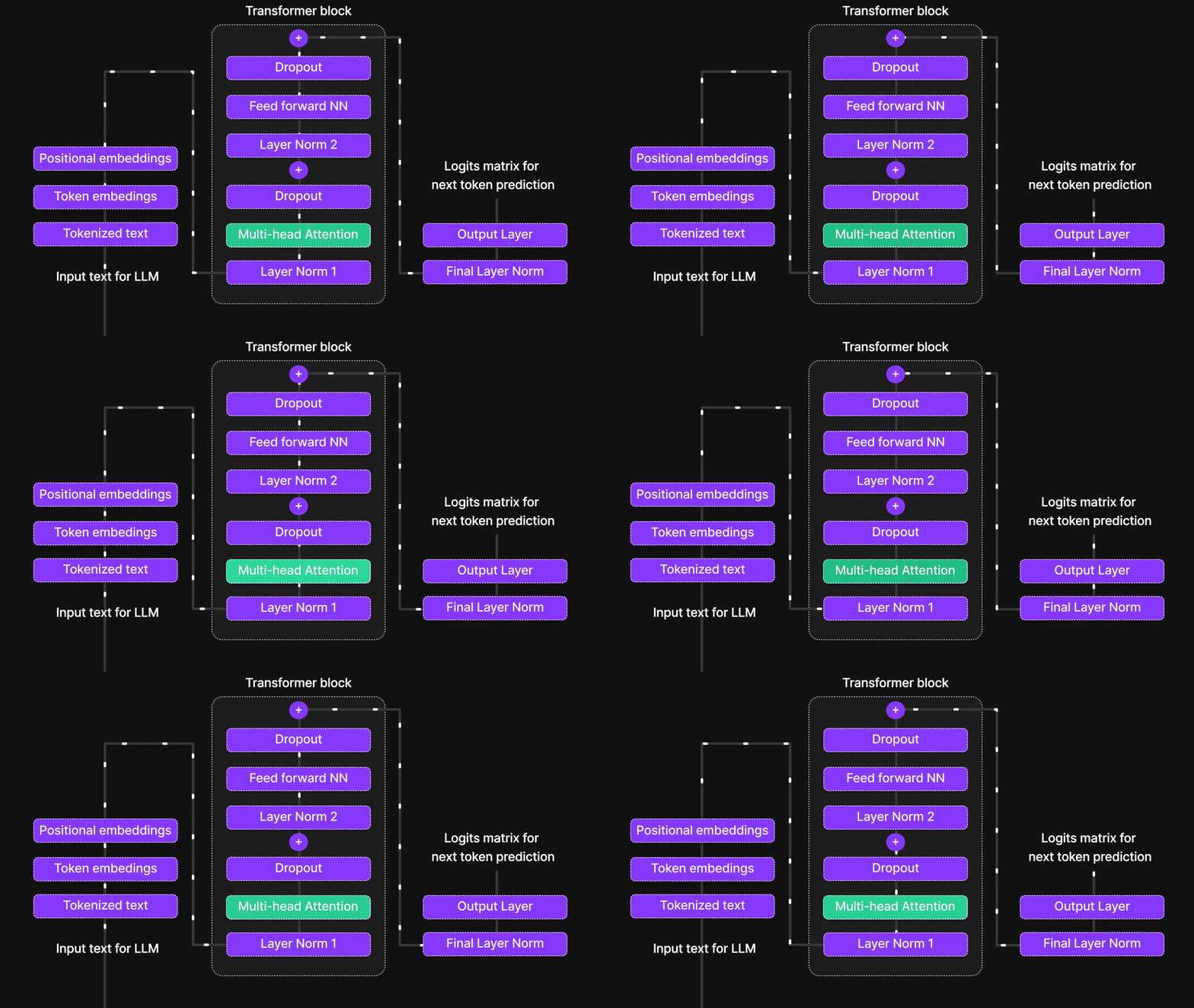Transformer Animation Source: Mayank Pratap Singh: The need of Attention Mechanism

Transformers convert input into tokens (numbers), where each token is represented as a vector called an embedding. In Vision Transformers (ViTs), images are likewise split into patches, each projected into an embedding. As these representations pass through the model, the goal is to make them increasingly rich by incorporating contextual information from other tokens. Attention blocks play a central role in this contextual refinement.

Each attention block contains multiple attention heads, where different heads capture different kinds of relationships between tokens. Modern transformer models stack many such attention blocks, continually refining token representations by injecting more and more contextual information. This structure is what allows transformers to model sequences so effectively and make strong predictions.

However, this continous refinement of token representations is also where our problem begins.

Think about it for a moment: do all tokens actually contain equal amounts of contextual information or require the same degree of updating? Consider punctuation tokens(. , / ? ), or special tokens such as beginning-of-sequence (BOS) or delimiter tokens (SEP). Similarly, in Vision Transformers (ViTs), many patches may contain very little useful information (e.g background regions like sky, walls, or empty spaces). Even semantically rich tokens may become “good enough” after passing through only a few attention blocks and may not require substantial further updates.

This naturally leads to an important question:

Does the transformer architecture allow token representations to stop updating once they become sufficiently good?

The Softmax Problem¶

Recall how attention is computed. Each token embedding is first projected into queries, keys, and values. The query of each token is then matched against all keys via dot products to produce similarity scores. These scores are normalized using a softmax, yielding attention weights (values between 0 and 1) that determine how much each token should contribute to the output. Finally, these weights are used to compute a weighted sum of the value vectors, producing the updated token representations. 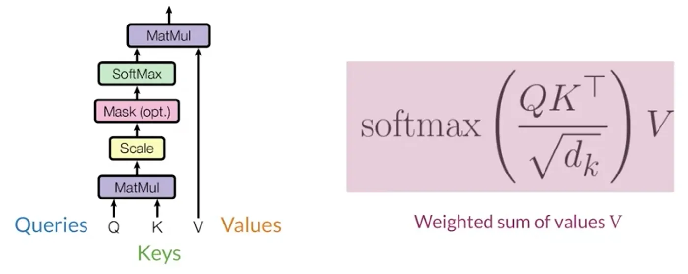Scaled Dot Product Attention Source: Bobby Cheng: The Why, What and Where of Transformers

Recall that the weights need to sum up to 1 (because of how softmax works). That’s the heart of the problem. The attention layer cannot simply “do nothing” - it must assign some amount of importance somewhere.

You might imagine a simple workaround: a token just focuses entirely on itself and ignores everything else. Unfortunately, this wouldn’t work because the attention output is always combined back with the original representation through the residual connection, and the representation itself gets updated by the value projection.

The Residual Connection Problem¶

Recall that in GPT-style models (pre-attention layer norm):

$$ x' = x + \mathrm{Attn}(\mathrm{LN}(x)) $$

Residual Connection

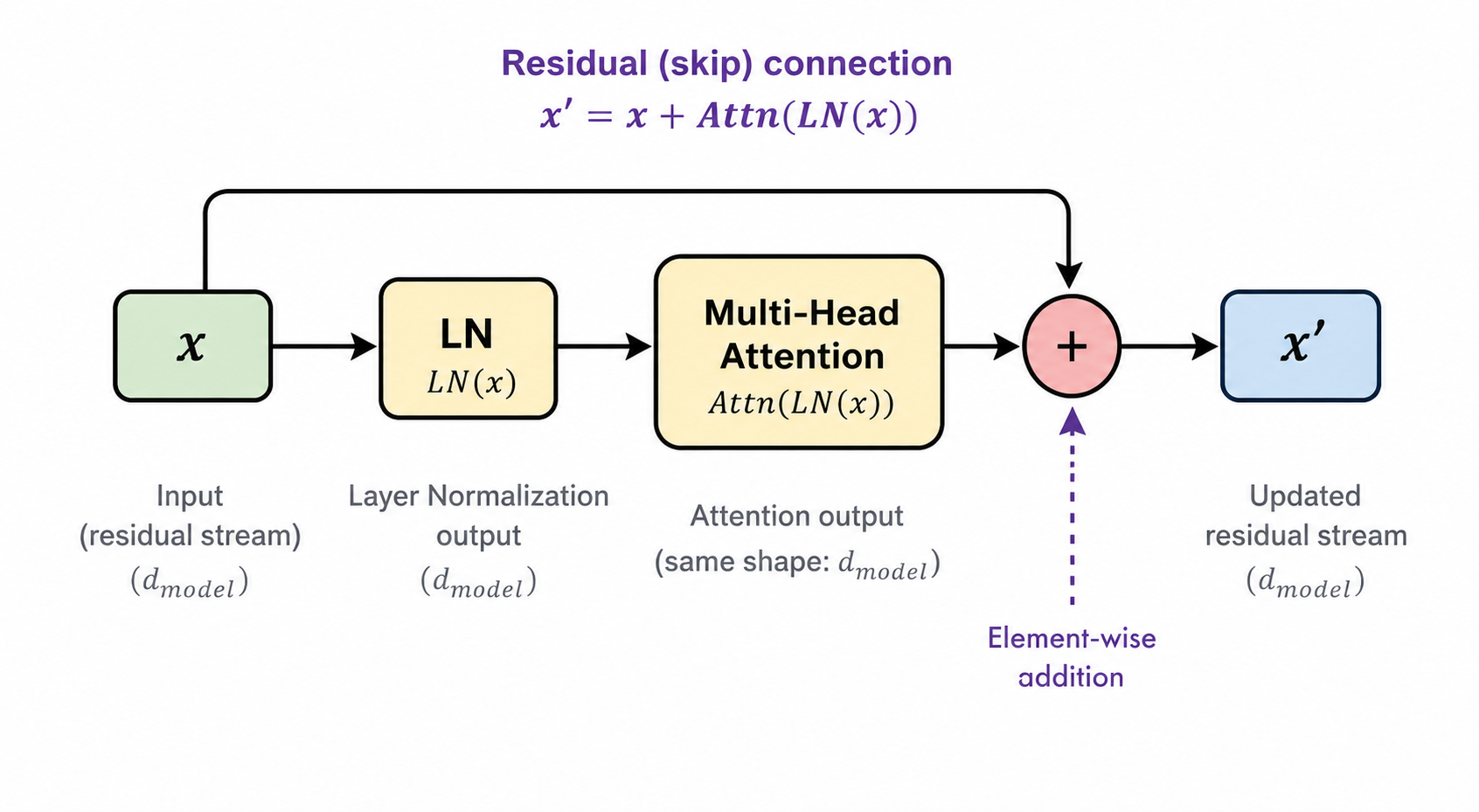
The “no-update” in this structure means attention does not need to preserve ( x ). It only needs to satisfy:

$$ \mathrm{Attn}(\mathrm{LN}(x)) \approx 0 $$

so that:

$$ x' = x $$

So, how does it work?

The Hack that Transformers Use¶

Recall that:

$$ \mathrm{Attn}_i = \sum_j \alpha_{ij} \cdot (V x_j) $$

Where:

$\alpha_{ij}$: attention weight from token (i) to token (j).
$x_j$: hidden representation.
$V$: value projection matrix.

We want:

$$ \mathrm{Attn}_i \approx 0 $$

Since the alphas cannot be all zeros, transformer models tend to assign large weights for tokens which have near-zero value vectors. These are generally tokens with low-semantic content e.g BOS tokens or delimiter tokens.

So, for certain tokens, if:

$$ V x_j \approx 0 \quad \text{(or very small norm)} $$

And if attention concentrates on such a token:

$$ \alpha_{ij} \approx 1 $$

then:

$$ \mathrm{Attn}_i \approx V x_j \approx 0 $$

The authors of the ICLR paper Efficient Streaming Language Models with Attention Sinks further found out that these are generally initial tokens & called them “Attention Sinks”. They hypothesized that, because autoregressive transformers allow every token to attend to earlier tokens, the initial tokens (e.g BOS token) are visible to the entire sequence and therefore become natural accumulation points for excess attention mass. As a result, these early tokens frequently emerge as stable attention sinks across many transformer models.

Note.

Strictly speaking, the full attention output involves an output projection matrix applied to the concatenation of all attention heads, giving the no-op condition: $$ W_O \begin{bmatrix} \mathrm{head}_1 \\ \vdots \\ \mathrm{head}_H \end{bmatrix} \approx 0. $$ This gives the model additional flexibility: in principle, a no-op could be achieved through cancellation across multiple heads rather than each head independently routing its attention to a sink token. However, empirical visualizations of attention patterns consistently show individual heads attending almost exclusively to BOS-like sink tokens.

But, what does all of this have to do with outliers?

The Chain Reaction¶

We’ve established that for a token to suppress its update, attention must concentrate disproportionately on a token with a near-zero value projection. The more mass concentrated on the sink, the smaller the residual update.

But how does softmax concentrate more mass on one token than the rest?

From the softmax equation, it is easy to see that this requires large logit gaps, i.e the sink token’s score must be significantly larger than the rest. The larger the gap, the more concentrated the distribution. Something like the middle row in the following example:

Softmax

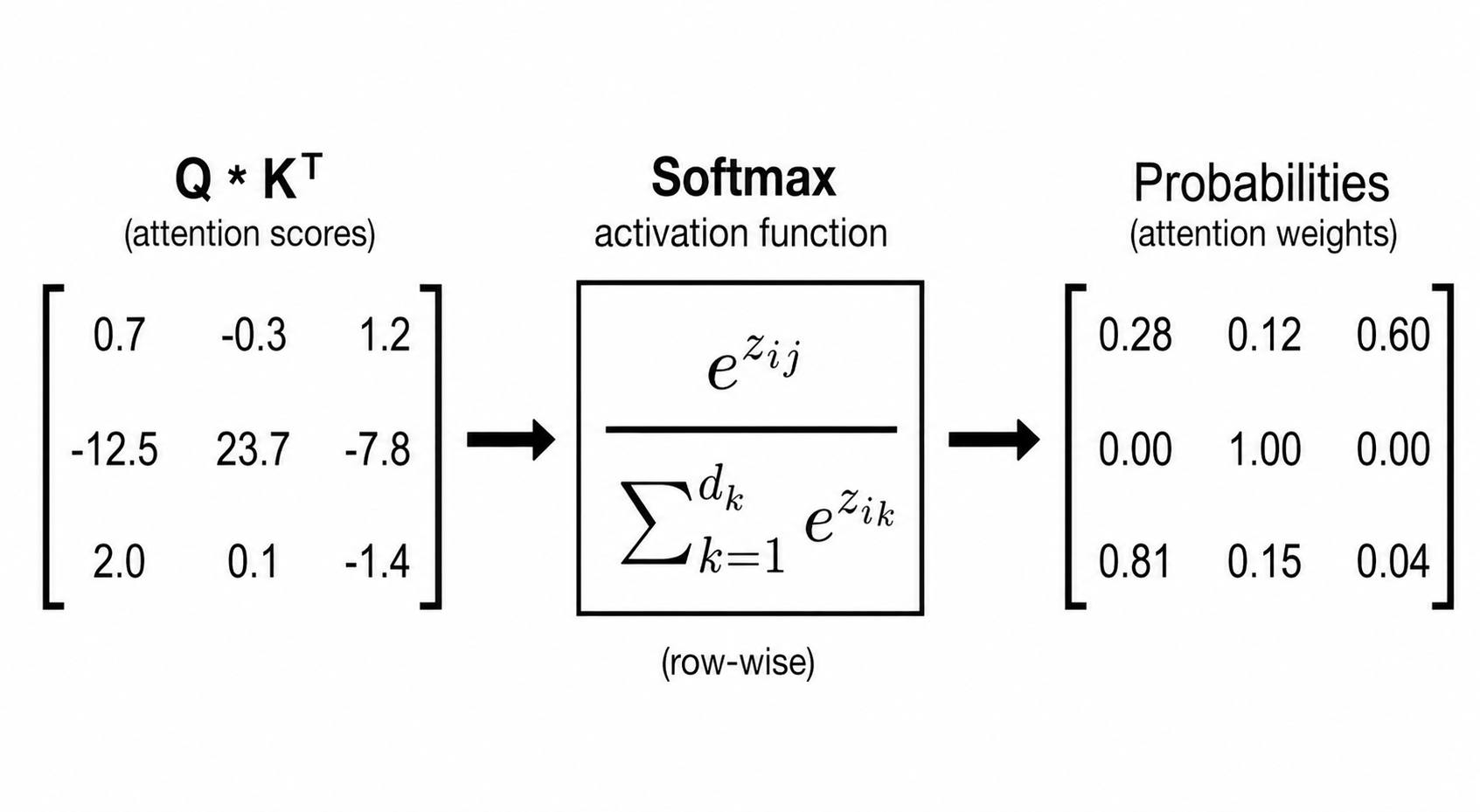
Mathematically, we want:

$$ q_i \cdot k_j \gg q_i \cdot k_t \quad \text{for } j \ne t $$

where:

$q_i$: query vector for token (i)
$k_j$: key vector for token (j)
. : dot product

Intuitively, a token that wants to suppress its update must match very strongly with an attention sink token while matching weakly with all other tokens.

From the definitions:

$$ q_i = W_q x_i, \quad k_j = W_k x_j, \quad k_t = W_k x_t $$

(Subscripts (i, j, t) index tokens, and (x)’s come from LayerNorm.)

Substituting:

$$ (W_q x_i) \cdot (W_k x_j) \gg (W_q x_i) \cdot (W_k x_t) $$

Using the dot product identity:

$$ a \cdot b = \|a\| \, \|b\| \cos \theta $$

we get:

$$ \|W_q x_i\| \, \|W_k x_j\| \cos \theta_{ij} \gg \|W_q x_i\| \, \|W_k x_t\| \cos \theta_{it} $$

Canceling the common term $\|W_q x_i\|$:

$$ \|W_k x_j\| \cos \theta_{ij} \gg \|W_k x_t\| \cos \theta_{it} $$

This inequality can be satisfied along two axes: by making the left-hand side large, or by keeping the right-hand side small. To understand what each requires, we need to answer two questions: what does LayerNorm do to token representations & how to interpret a matrix-vector product?

Normalization¶

Recall that LayerNorm normalizes each token using the mean and standard deviation computed across its embedding dimension, before applying a learned per-dimension scale and shift:

$$ x_k \rightarrow \gamma_k \frac{x_k-\mu}{\sigma} + \beta_k. $$

Ignoring the affine transform $(\gamma,\beta)$ for the moment, the squared norm of the normalized token is

$$ \left\| \frac{x-\mu}{\sigma} \right\|^2 = \frac{1}{\sigma^2} \sum_k (x_k-\mu)^2 = d, $$

since

$$ \sigma^2 = \frac{1}{d} \sum_k (x_k-\mu)^2. $$

Thus, every normalized token has the same Euclidean norm, $\sqrt{d}$, and lies on a hypersphere of radius $\sqrt{d}$.

The learnable affine transform

$$ y = \gamma \odot \hat{x} + \beta $$

distorts this geometry, but it is shared across all tokens and therefore cannot make a token’s output magnitude larger simply because its input magnitude was larger.

Consequently, a sink token cannot obtain a large $\|W_Kx_j\|$ merely by entering LayerNorm with a large norm. Therefore, any systematic differences in $\|W_Kx_j\|$ must instead arise from the token’s direction (i.e., its feature pattern), not its original magnitude.

What a linear map does to a vector¶

A linear transformation

$$ x \mapsto Wx $$

can always be decomposed (via SVD) into three steps:

$$ W = U S V^\top $$

where:

$V^\top \in \mathbb{R}^{d_{\text{in}} \times d_{\text{in}}}$ is an orthogonal rotation
(it changes directions but not lengths or angles).
$S$ is a diagonal matrix of non-negative singular values

$$ \sigma_1 \ge \sigma_2 \ge \cdots \ge 0 $$

It stretches/compresses each axis independently.

$U \in \mathbb{R}^{d_{\text{out}} \times d_{\text{out}}}$ is a second rotation, giving the final orientation.

Thus, applying $W$ to a vector $x$ consists of:

Rotate $x$ by $V^\top$
This re-expresses $x$ in the “principal” coordinate system of $W$.
Scale each coordinate by the corresponding singular value $\sigma_i$
If $x$ happens to align with a singular vector with a large $\sigma$, the output norm becomes much larger than the input norm. If it aligns with a small $\sigma$ (or is orthogonal to large ones), the output becomes tiny.
Rotate the result by $U$
This gives the final output direction.

Satisfying the inequality¶

With both pieces in place, the dominance condition becomes a statement about directions:

Left-hand side: For $\|W_k x_j\| \cos \theta_{ij}$ to be large, two things must hold simultaneously. First, the sink token’s representation $x_j$ must align strongly with the high-singular-value directions of $W_k$, so that the key vector $k_j$ = $W_k x_j$ has large norm. Second, the query $q_i$ must point in the same direction as $k_j$ for $\cos \theta_{ij}$ to be large. Since $k_j$ is the output of $W_k$, its direction is determined by $W_k$’s dominant singular structure. For $q_i$ to reliably land in that same direction, $W_q$ must strongly amplify it too. This is the core constraint: $W_q$ and $W_k$ must develop overlapping dominant singular subspaces, i.e they must agree on which directions to amplify.
Right-hand side: For $q_i⋅k_t$ to remain small for all ordinary tokens $k_t$, those tokens’ key vectors must not overlap with those directions. Therefore, the model achieves this by reserving a small set of specialized high-magnitude directions exclusively for the no-op mechanism.

Taken together, both conditions force the model to concentrate representational energy into a small number of disproportionately amplified directions. In weight space, this shows up as a few rows or columns of $W_q$ and $W_k$ with anomalously large magnitude. In activation space, when inputs pass through these weight matrices, a small number of feature dimensions carry values far larger than the rest. These are the outlier channels. But once they form, what keeps them there?

Training Dynamics:¶

Once outlier channels exist, training actively reinforces them. Softmax with a near-one-hot distribution has gradients concentrated almost entirely on the dominant logit — the one produced by the outlier dimensions. The gradient signal flowing back into $W_q$ and $W_k$ is therefore concentrated in precisely those outlier directions, making them stronger with each update.

LayerNorm compounds this. Because it suppresses global scale and equalizes norms across tokens, upstream MLPs must produce outputs large enough that the outlier signal survives normalization and generates sufficient dynamic range for softmax. This pushes earlier layers to amplify outlier dimensions further.

The result is a self-reinforcing loop: outlier channels produce sharp softmax distributions, sharp distributions concentrate gradients back into outlier channels, and the cycle repeats across training.

Therefore, outliers are not isolated phenomena; they emerge systematically and are interconnected across multiple dimensions within the model. The ICLR paper, Sytematic Outliers in Large Language Models studied how weight outliers give rise to activation outliers, which in turn propagate into attention outliers for Llama 2 7B.

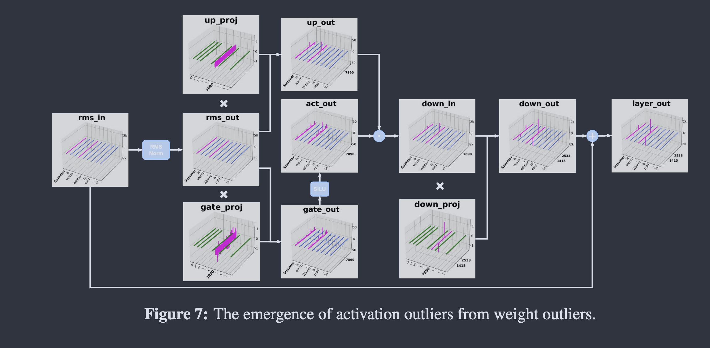
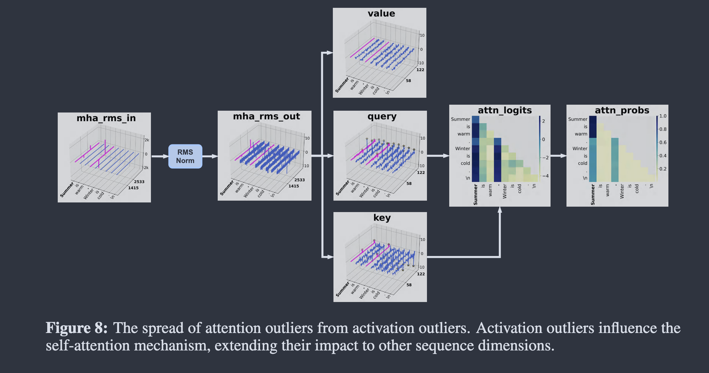
Activation Outliers from Weight Outliers

Attention Outliers from Activation Outliers

Source: Systematic Outliers in Large Language Models

Conclusion¶

Thank you for reading! I hope it gave you some useful intuition about why outliers are so prevalent in transformer models. In summary, they emerge from the attention mechanism’s inability to perform a no-op directly due to the sum-to-one constraint of softmax, and once they exist, they are actively reinforced during training. In the next post, we’ll discuss why this makes quantization hard and cover some of the early breakthroughs that first unlocked outlier-aware quantization.

References & Further Reading¶

Quantizable Transformers: Removing Outliers by Helping Attention Heads Do Nothing: The first paper to identify that outliers emerge due to the sum-to-one constraint of softmax. The authors also propose a “Clipped Softmax” and a “Gated Attention” function which, in their experiments, prevent the formation of outliers. Wider adoption remains to be seen.
Attention Is Off By One: Evan Miller read the above paper and suggested a simple tweak to the softmax formula: adding a 1 to the denominator so that the weights no longer need to sum to 1. This gained a lot of traction when it was released but has not seen practical adoption.
Systematic Outliers in Large Language Models: The authors do a systematic analysis of outliers by defining weight outliers, activation outliers, and attention outliers, and study how each gives rise to the next. They also evaluate various attention variants to find out how to prevent outlier formation, and find that a learnable scaling factor that dynamically adjusts attention weights (Explicit Context-Aware Scaling) does not lead to outlier formation. Wider adoption remains to be seen.
Attention Is Not All You Need: Not directly related, but since this post discusses a subtle limitation of the standard attention mechanism, you may find this one interesting. The authors show that if you have only attention layers with no MLPs or residuals, the output converges to a rank-one matrix with identical rows at a doubly exponential rate. MLPs and residual connections fight against this. So the residual connection doesn’t just help with gradient flow, it also fights to prevent representational collapse.