Machine Learning (ML) has witnessed a surge in interest in recent years driven by the availability of large-scale datasets, advances in ML frameworks such as PyTorch and TensorFlow, rise of hardware accelerators (e.g., GPUs and TPUs) that enable large-scale training, and the development of increasingly powerful neural network architectures. Together, these factors have enabled the creation of highly capable models with wide ranges of applications.
Scaling Laws have demonstrated model performance improves predictably with the increase in model size, dataset size and compute. This has led companies to train even larger models on massive datasets, requiring a vast amount of computational resources. As a consequence, it is expected that the cost of training models will rise from $100 Million to $500 Million by 2030. At the same time, International Energy Agency projects that the energy requirement for AI could double over the same period.
Beyond training costs, deployment introduces another critical constraint for these models: user experience. Models must operate with low latency & high throughput to be practical in real-world applications. Therfore, it has become increasingly important to develop techniques to optimize these models and make them faster, greener and more cost efficient.
Enter Model Compression.
Model compression refers to a set of algorithms that aim to reduce the size, memory and power requirements of neural networks without significantly impacting their accuracy. These include pruning redundant connections in the model, representing the parameters through lower precision datatypes, exploiting the structure of data to represent the layers more efficiently, or training smaller and more efficient models.
The goal of this blogpost is to provide a high-level overview of these techniques.
Quantization: Making the most of approximations
What is Quantization?
Modern models are typically trained using mixed precision, i.e some operations in float16 or bfloat16, and others in float32. As a rule of thumb, a model with N billion parameters requires roughly 2 × N GB of memory when stored in 16 bits. For instance, a 3B parameter model needs about 6 GB of memory, a 7B model needs 14 GBs and so on.
Quantization reduces this footprint by representing weights and activations using lower-precision data types such as int8, effectively halving memory requirements. Beyond memory savings, prior work (e.g., Horowitz, 2014) has showed that integer arithmetic is generally faster and more energy-efficient than floating-point computation.
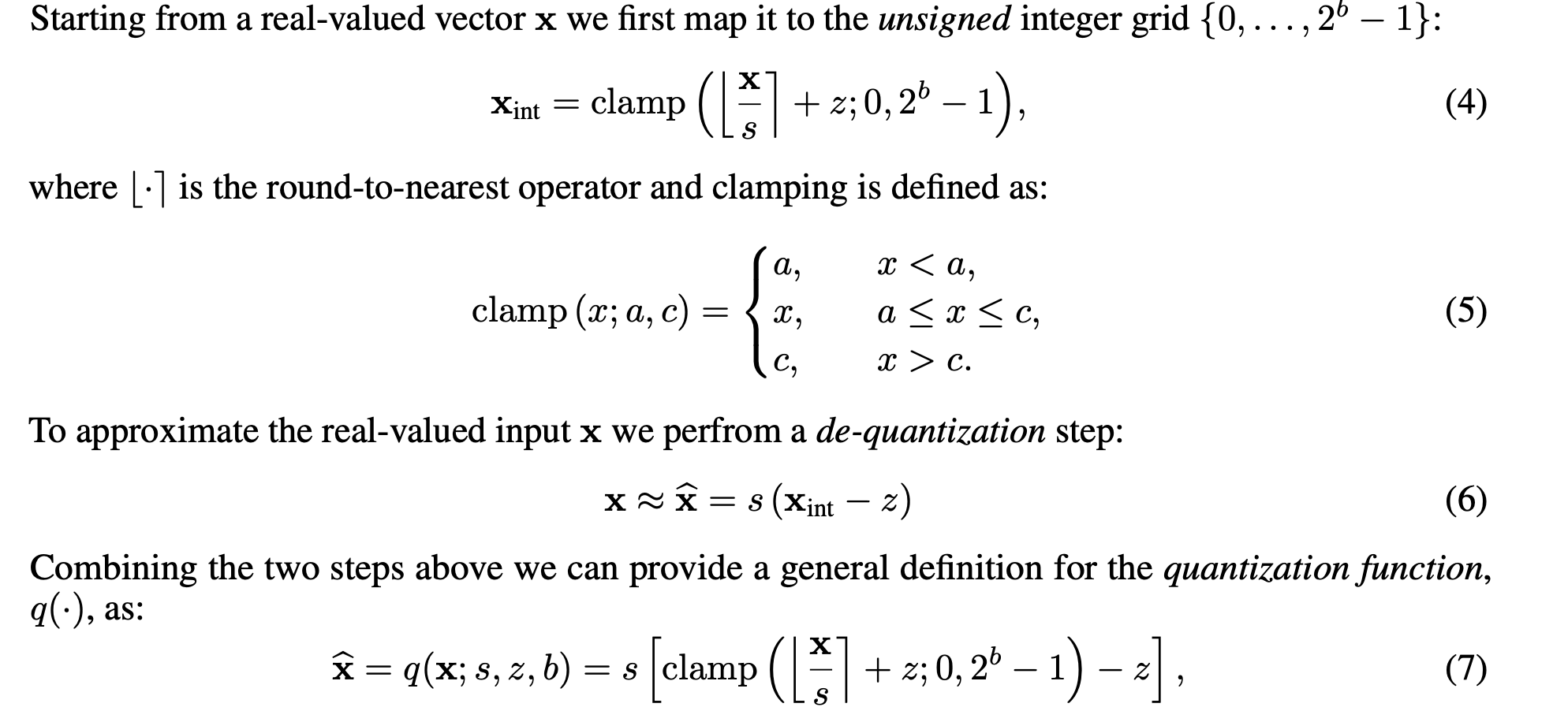 Quantization Steps: Source: A White Paper On Neural Network Quantization
Quantization is therefore a key model compression technique for efficient deployment of neural networks on mobile phones and other resource-constrained edge devices.
What are the different types of quantization algorithms?
Quantization can be categorized along several axes, depending on when it is applied, how parameters are represented, and how computations are performed.
Based on when it is applied: During Training or Inference?
Quantization aware training (QAT) simlutes inference-time quantization duering training by using quantized weights and activations in the forward pass, while using full precision weights in the backward pass. The idea is to emulate the inference time quantization error by using quantized values in the forward pass, and allowing the backward pass to update the full-precision weights such that they become more robust to quantization. This approach leads to better accuracy preservation as the model learns to adapt to the precision loss during training.
Quantization Aware Training. Source: Quantization and Deployment of Deep Neural Networks on Microcontrollers
Unlike quantization aware training, where the model learns to adjust to lower precision during training, post-training quantization (PTQ) directly applies this reduction in bit width after the model has been trained. While it may not offer the same level of accuracy preservation as quantization aware training, it is widely used in practice since it doesn’t require retraining the model.

Post Training Quantization. Source: Practical Quantization in PyTorch
Based on how quantization parameters are applied:
- Per-tensor quantization: a single scale and offset are used for the entire tensor.
- Per-channel quantization: each channel has its own scale and offset.
- Block quantization: groups of elements share quantization parameters.
In general, finer-grained schemes (more parameters) yield better accuracy but introduce additional storage and compute overhead.
Based on how activations are quantized:
Since weights are always known before inference they can be quantized offline, however, activations depend on the input to the model, and there are two ways of quantizing them.
In static quantization, the min and max ranges of activations are calculated using a small subset of the training data called calibration dataset which typically contains around 300-500 samples. This technique is typically used when both memory bandwidth and compute savings are important with CNNs being a typical use case.
In dynamic quantization, the min-max ranges are calculated on the fly during inference. This is useful in situations where the model execution time is dominated by loading weights from memory rather than computing the matrix multiplications. For example, this is true for LSTM and Transformer type models with small batch size.
Based on quantization mapping:
Affine quantization incorporates scaling (Scale S) and a non zero shifting(Zero Point Z) allowing for a flexible representation of a wide range of values by adjusting magnitude and position before rounding.
Symmetric quantization is a special case of affine quantization where-in the values are mapped to a symmetric range of values i.e [-a, a]. In this case, the integer space is usually [-127, 127], meaning that the -128 is opted out of the regular [-128, 127] signed int8 range. The reason is that having both ranges symmetric allows to have Z \= 0. While one value out of the 256 representable values is lost, it can provide a speedup since a lot of additional operations can be skipped.
Pruning: Keeping what matters
What is Pruning?
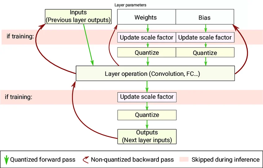
Pruning is a model compression technique that involves removing redundant or less important weights from a neural network to reduce model size and compute while preserving accuracy. Typically, weights are pruned based on critera such as magnitude or their estimated impact on the model’s output.
A neural network structure, before and after pruning. Source: Learning both Weights and Connections for Efficient Neural Networks
What are the different types of pruning algorithms?
Pruning can also be categorized along several dimensions:
Based on how weights are removed
- Unstructured pruning: removes individual weights without constraints, resulting in sparse weight matrices. While this can achieve high compression, it often requires specialized hardware or libraries to realize speedups.
- Structured pruning: removes entire structures such as neurons, channels, or filters. This produces dense, smaller models that are more compatible with standard hardware and typically lead to practical speedups.
- Semi-structured pruning : imposes regular sparsity i.e N:M patterns. For example, 2:4 sparsity, where for every group of 4 weights 2 are zeroed out. It’s a middle ground between structured and unstructured pruning and provides real speed ups (e.g on Nvidia sparse tensor cores.)
Based on how pruning is performed?
- One-shot pruning: removes weights in a single step. It is simple but can lead to significant accuracy degradation.
- Iterative pruning : gradually removes weights over multiple steps, often interleaved with fine-tuning. This approach generally preserves accuracy better.
Based on scope
- Local pruning: applies pruning independently within each layer.
- Global pruning: selects weights to prune across the entire network based on a global criterion, often leading to better overall allocation of sparsity.
Tensorization / Factorization: Higher ranking doesn’t mean better
What is Tensorization / Factorization?
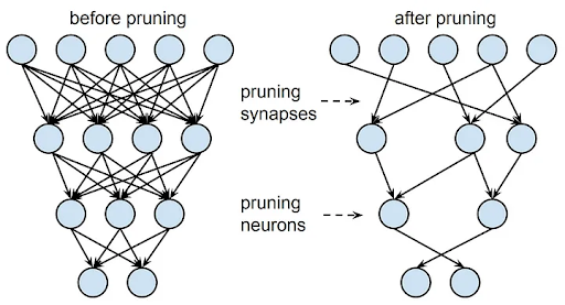
Tensorization (or factorization) decomposes weight tensors into lower-rank components, reducing parameter count while preserving the most important structure in the data.
Visual representation of the tensorization process applied to image data. Source: Tensor Contraction and Regression Networks
What are the different types of tensorization/factorization algorithms?
There are four popular tensor decomposition algorithms which are used extensively:
- Singular Value Decomposition: Decomposes a matrix A into UΣV⊤, where a low-rank approximation retains only the top singular values. This provides the most optimal rank-r approximation of the matrix (Eckart-Young theorem). It is directly applicable to 2D weights (e.g., linear layers); higher-dimensional tensors must be reshaped.
- Canonical Polyadic Decomposition (CP or PARAFAC): Factorizes a tensor into a sum of rank-1 tensors. Each component captures a separable pattern across all modes, enabling direct decomposition of multi-dimensional weights without flattening.
- Tensor Train Decomposition : Represents a high-dimensional tensor as a sequence of smaller, interconnected tensors (“cores”). This factorization scales linearly with the number of dimensions, making it efficient for very large tensors.
- Tucker Decomposition: Decomposes a tensor into a smaller core tensor multiplied by factor matrices along each mode. It can be seen as a higher-order generalization of SVD, allowing different ranks per dimension.
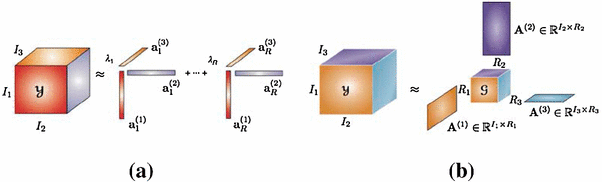 Visual representation of CP & Tucker Decomposition. Source: Research Gate
How is Tensorization used in practice?
Tensorly is the most popular library for working with tensor decompositions. It works with various frameworks such as Numpy, Pytorch and TensorFlow & provides off-the-shelf API for all the algorithms we discussed. Extending the core features of TensorLy, TensorLy-Torch provides out-of-the-box tensor layers that can be used to implement and train tensorized networks from scratch or fine-tuning existing models by replacing the layers with their tensorized counterparts. Some examples are:
- Factorized Convolutions: which decompose the convolution filter into two or more smaller filters, reducing parameter count and compute.
- Tensorized Linear Layers: where the 2D weight matrix of a linear layer is first tensorized (reshaped into a higher dimensional tensor) and then factored using a high-dimensional decomposition / tensorization method.
- Factorized Embedding Layers: which can act as a drop-in replacement for Pytorch’s embeddings but using efficient tensor parametrization that doesn’t need to reconstruct the table.
- Tensor Regression Layers: eliminate fully connected layers by regressing directly on convolutional activations using low-rank tensor factorization.
Knowledge Distillation: Why reinvent the wheel?
What is Knowledge Distillation?
Knowledge distillation involves transferring knowledge from a complex, large model (teacher network) to a smaller, simpler neural network (student model). The goal here is to leverage the knowledge learned by a large model to train a small model to mimic it’s behavior.
At a high-level, knowledge distillation involves two main steps:
-
Training the teacher model: Involves training the teacher network to a desired level of accuracy
-
Training the student model: Using the outputs of the teacher network as soft targets i.e probability distributions over the classes instead of hard labels
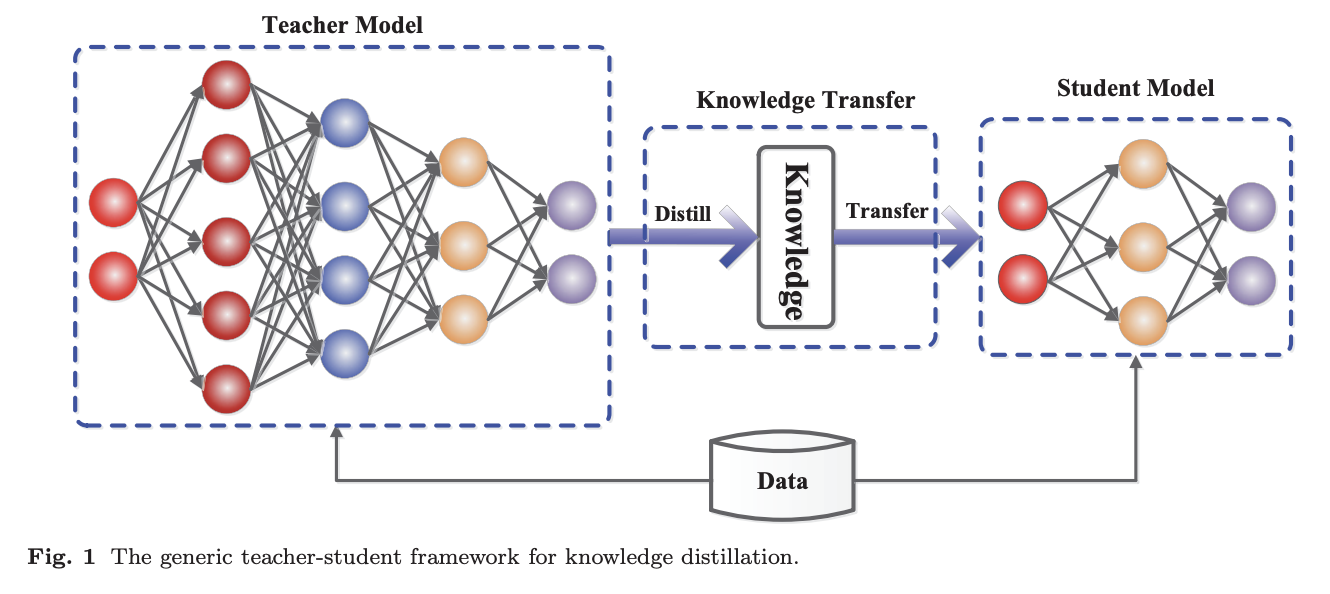 An illustration of the knowledge distillation process. Source: Knowledge Distillation: A Survey
What are the different types of knowledge distillation algorithms?
Knowledge Distillation techniques generally pertains to one of the following categories:
- Offline Distillation: is the most common distillation technique and involves using a trained model (teacher) to guide another smaller model (student).
- Online Distillation: is used when a trained teacher model isn’t available. In online distillation, both teacher and student models are updated simultaneously in a single end-to-end training process.
- Self Distillation: is a special case of online distillation and involves using the same model as the teacher as well as the student. In self-distillation, knowledge from deeper layers of the network is used to guide the shallow layers.
Conclusion
Models may keep scaling, but so do the bills. Model compression is how we push back. Hope this gave you a useful overview. Thank you for reading!